
Most grow rooms can already dim. What they cannot always do is hold a light target. A schedule that sets fixtures to 70% on day one delivers something close to the intended photon flux; the same 70% three seasons later delivers less, because the emitters have aged, the covers have accumulated dust, the driver has drifted with temperature and the reflective surfaces have been washed or replaced. The controller believes it is at 70% because that is what it commanded. Nothing in the loop has measured light.
Closed-loop control replaces the assumption with a measurement. This article covers what such a loop actually reads, where the quantum sensor belongs, how the daily light integral is accumulated and converged before sunset, which control law keeps the loop stable, how ramping protects both plants and hardware, and where the communication layer sets hard limits on what any controller can achieve.

Open-Loop Dimming and Why It Drifts
An open-loop system maps a command to a duty cycle and assumes the resulting photon flux is proportional. That assumption fails in four predictable ways: luminous depreciation of the LEDs, contamination of the emitting surface and any cover, thermal drift in the driver’s current regulation, and changes in the reflective environment around the canopy when walls are re-clad, trays are added or a neighbouring zone is reconfigured.
Depreciation is the largest term and it is specified, not accidental. A fixture rated to L90 is permitted to fall to 90% of initial output within its rated hours; one rated to L70 is permitted to fall to 70%. That means an open-loop room can be running at 10–30% below its design PPFD at end of life while the controller still reports 70%. Soiling adds a further few percent at each cleaning interval, depending on airflow, irrigation method and whether the cover is horizontal and upward-facing.
The two errors compound rather than cancel. A fixture at 85% of initial output behind a cover transmitting 92% delivers about 78% of nameplate flux, so a 300 µmol/m²/s setpoint silently becomes 234 µmol/m²/s. Over a 16-hour photoperiod that is a daily light integral shortfall of roughly 4 mol/m²/d — enough to change rooting time, stretch and flowering response in many crops. Nobody sees it in the control dashboard, which is the defining weakness of an open loop.
What a Closed Loop Actually Measures
A closed loop inverts the relationship: a sensor measures photon flux density at a reference plane, the controller compares that reading with a target, and the dimming command is adjusted until the error is inside a deadband. The command becomes an output of the loop rather than an assumption about the hardware.
There are two common architectures. The first places the sensor on a fixed bracket in the canopy plane and treats the reading as representative of the zone; this is cheap and stable, and it converges on whatever the sensor sees, including its own placement error. The second uses multiple sensors or a roving measurement to characterise the zone and applies a correction factor per luminaire group.
What the loop cannot do is infer canopy flux from a ceiling-mounted reading. A sensor near the fixtures tracks output rather than what the crop receives, and the measurement plane should match the decision plane: if the target is canopy PPFD, the sensor belongs at the canopy.
Sensor Placement and Cosine Error
Placement dominates accuracy, and the parameter that most often goes unstated is the cosine response. A quantum sensor should measure the flux from a hemisphere weighted by the cosine of the incidence angle; real diffusers deviate, and a cosine error of 3% or less is a reasonable specification for a horticultural-grade instrument. A sensor with worse cosine response misreads a side-mounted high-angle beam differently from an overhead one, so its error changes whenever fixtures are re-aimed; the photobiology work at Utah State University’s Crop Physiology Laboratory is a useful reference point for how these measurements are handled in practice.
Height and angle should be fixed and documented. A common convention is 0.3–0.5 m above the canopy top, or the distance specified by the instrument maker, on a bracket that is levelled and stays levelled. The sensor must not sit in the shadow of a truss, a fan or an irrigation pipe, and must not sit under a fixture’s hotspot if the zone average is the target. Where a single sensor serves a large bay, the reading is a sample, and sampling error can exceed the drift the loop was installed to correct.
Calibration is a maintenance item with a schedule, not a one-time step. A 6–12 month interval is typical, and recalibration is mandatory after any lamp or driver replacement, after a sensor is moved, and after a cover is cleaned or changed. A drifted sensor produces a drifted loop that looks perfectly healthy on the dashboard — the most expensive failure mode in the whole system, because it is invisible.
From PPFD to DLI: The Daily Integral
The daily light integral is the integral of PPFD over the photoperiod, expressed in moles per square metre per day: DLI = PPFD (µmol/m²/s) × 3600 × photoperiod (h) / 1,000,000. A room held at 300 µmol/m²/s for 16 hours delivers 17.3 mol/m²/d; the same room at 200 µmol/m²/s for 12 hours delivers 8.6. The definition and the role of supplemental lighting in raising it are set out in extension guidance such as Michigan State University’s note on daily light integral and its guidance on maximising supplemental lighting.
Targets are crop-specific and should be quoted with the crop attached. Leafy greens are commonly grown in the range of about 12–17 mol/m²/d, fruiting crops in the range of about 15–25 mol/m²/d, and propagation is usually run lower to limit stretch. Cultivar, temperature, CO₂ and the natural light available all shift the number, which is why a controller should store DLI targets per zone and per crop cycle rather than as a single site-wide constant.
Because DLI is an integral, a closed loop has to reason about the remaining time, not just the current error. The standard approach accumulates delivered moles through the day, then computes the PPFD needed to close the gap over the hours left: required PPFD = (target − accumulated) × 1,000,000 / (3600 × remaining hours). With a 14 mol target, 8 mol already delivered by mid-afternoon and 4 hours of photoperiod left, the loop needs 416 µmol/m²/s for the remainder — a step that is entirely feasible in a well-designed room.
The step must be bounded. Every crop has a PPFD level above which additional photons stop paying for themselves and photoinhibition or heat load becomes the constraint, so the controller needs a hard ceiling that outranks the DLI target. A loop that chases the integral without a ceiling will, on a short winter day, push fixtures to full output at the worst possible moment and deliver stress instead of growth. The correct behaviour is to miss the target and log the shortfall.
Control Law: PI, Deadband and Anti-Windup
The simplest loop is a threshold switch: if the reading is below target, raise the command; if above, lower it. Bang-bang control is cheap and it oscillates, because the command steps across the target repeatedly and the room sees a square wave of light at the loop period. In a plant canopy that oscillation is mostly harmless; in the electrical and thermal domain it is not, since drivers cycle and the measured average drifts with the loop’s duty cycle.
Proportional-integral control is the usual upgrade. The proportional term responds to the current error, the integral term removes steady-state offset, and a deadband of a few percent around the target prevents the loop from hunting on sensor noise. The integral term needs anti-windup: when the output is already at 100% and the error persists, the integral accumulates and then overshoots when conditions change, driving the command to full for minutes after the need has passed. Clamping the integrator whenever the output saturates, or freezing it inside the deadband, removes most of that behaviour.
Sampling interacts with the control law more than most commissioning teams expect. A sensor sampled every 1–10 s and smoothed with a 1–5 minute moving average gives a stable input, and command updates at 60 s or slower suit a target that changes over hours. Faster loops buy nothing except sensitivity to a cloud passing over a vent.
Photoperiod Ramping and Transition Safety
Switching a room from 0 to 100% in one step is electrically convenient and biologically abrupt. A ramp of 15–30 minutes at each end of the photoperiod spreads the transition, which matters for two reasons: the crop is not exposed to a step change in irradiance and leaf temperature, and the fixtures themselves avoid the thermal and condensation shock of a cold start in a humid room.
Ramping also interacts with the DLI calculation. If the first and last 20 minutes of the photoperiod are ramped, the delivered integral is slightly lower than a rectangular profile of the same nominal length, so the loop should integrate the measured PPFD rather than assume the setpoint. This is one of the practical arguments for closed loop over schedule: the controller measures what actually happened, including its own ramps.
At the end of the day the ramp should converge the integral, not truncate it. A loop that schedules a ramp-down at a fixed clock time will cut off whatever the day delivered; a loop that ramps down when the accumulated integral reaches the target, or when the photoperiod expires, keeps the daily dose repeatable across seasons.
Protocol Limits: 0–10 V vs DALI-2 vs Wireless Mesh
The communication layer sets a hard floor on loop period and a hard ceiling on zoning. A 0–10 V analog interface is unidirectional and unaddressed: the controller sends a voltage, every driver on that circuit follows it, and nothing is read back. There is no way to confirm that a fixture received the command, and no way to correct one fixture independently of its neighbours. Closed loop on 0–10 V therefore works only at the granularity of the whole circuit, and only if the sensor is positioned to represent that circuit.
DALI-2 is addressable and bidirectional: fixtures can be commanded individually and their actual dimming level can be read back, which allows a controller to distinguish “commanded” from “achieved” and to detect a driver that has failed or drifted out of calibration. Zoning becomes a software decision rather than a wiring decision, and per-bay correction becomes possible without extra cabling.
Wireless mesh sits between the two on capability and behind both on determinism. It supports addressing and readback in principle, but latency, retries and occasional packet loss mean the loop period must be conservative and the control law must tolerate missing samples. A mesh loop designed around a 1-minute period with a deadband and a filtered input behaves well; one designed around a 5-second period will spend its time recovering from dropouts.
Independent of protocol, the loop period should be at least 1 minute, because it has to include sensor sampling, filtering, the control calculation and command dispatch. Anything faster is measuring the transport rather than the crop.
Control Architecture Comparison
The table compares the practical architectures. Loop periods are typical commissioning values rather than protocol limits, and the failure modes are the ones that actually appear in service.
| Control architecture | Reads back measured PPFD | Typical loop period | Zoning capability | Main failure mode | Typical application |
|---|---|---|---|---|---|
| Open loop, percentage schedule | No | Not applicable | Per circuit by wiring | Silent drift from depreciation, soiling and driver tolerance | Low-value propagation, short cycles |
| Single-point closed loop on 0–10 V | Yes, one point | 1–5 min | Whole circuit only, no addressing | Sensor misplacement or drift controls the entire zone | Single-bay rooms with uniform canopy |
| Multi-point grid with DALI-2 | Yes, 4–9 points per zone | 1–2 min | Per luminaire group, software-defined | Commissioning complexity; address mapping errors | Multi-zone rooms, research and phenotyping |
| Wireless mesh closed loop | Yes, with dropouts | 2–10 min | Per node, latency-dependent | Packet loss and retries destabilise fast loops | Retrofits where cabling is impractical |
The single-point row is the one most often installed and the one most often misconfigured: it does read back, so it looks like a closed loop, yet a sensor in the wrong place simply locks the room onto a wrong number with great precision. The DALI-2 row is the only one that can separate a fixture-level fault from a zone-level shortfall.
Commissioning Checklist
- Fix sensor height, angle and bracket position, and record them on the zone drawing before the first calibration.
- Calibrate against a reference instrument, log the date and the correction factor, and schedule the next calibration 6–12 months out.
- Measure a grid of 4–9 points at canopy level and record the spread; if the spread exceeds roughly 10%, the zone needs re-aiming before the loop can be trusted.
- Set the DLI target per zone and per crop, with an explicit PPFD ceiling that outranks the target.
- Configure the deadband, the ramp duration and the dim floor, and document the intended behaviour when the target cannot be met.
- Log at least: timestamp, zone, measured PPFD, commanded level, achieved level where readback exists, accumulated DLI, and any saturation flag.
- Run one full photoperiod in monitor-only mode before enabling feedback, and compare the logged integral with the hand calculation.
Where Closed-Loop Control Pays Off
The economics of a closed loop depend on how much drift the room can tolerate. In a research or phenotyping facility, where treatments must be repeatable across benches and cycles, closed loop is not optional — it is the only way to demonstrate that two plots received the same dose. In a commercial leafy-green room running continuous cycles, the value is in holding the integral steady as fixtures age and covers soil, so that harvest timing does not creep.
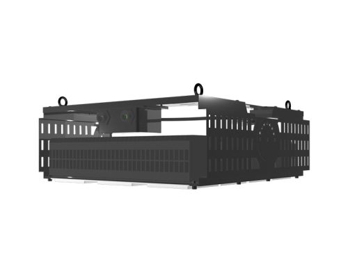
Koray has been manufacturing horticultural lighting for 17 years, and the practical request we see most often is not for a controller but for the measured data to commission one: what the fixture delivers at a given dim level, at a stated distance, with the production cover fitted. The G4000H module and G630 top light families are typically paired with an addressable dimming layer where zoning matters, and with amplitude dimming where the low end of the range has to stay free of visible modulation — the percent-flicker behaviour of a PWM stage below 10% is the one cross-check worth carrying over from the flicker literature, and the U.S. DOE briefing on IEEE 1789 is the reference for how that boundary moves with frequency.
Common Mistakes
- Treating the commanded percentage as a PPFD value, and reporting it as if it were measured.
- Sampling a single point under a hotspot and calling it the canopy average.
- Chasing the DLI target past the crop’s PPFD ceiling on short days.
- Running a fast loop over a wireless mesh and interpreting dropouts as a crop response.
- Using one 0–10 V circuit for several zones and expecting per-zone correction.
- Skipping the monitor-only commissioning day, then discovering the sensor was inverted.
Conclusion
Closed-loop PPFD and DLI control is a measurement discipline before it is a hardware purchase. The loop is only as good as the sensor’s placement and calibration, the integral only as good as its ceiling, and the control law only as stable as its anti-windup and its loop period. A room that logs measured PPFD, commanded level and accumulated DLI can prove what the crop received; a room that logs a percentage cannot, however precise the number looks.
Frequently Asked Questions
Do I need a PAR sensor per tray?
Not per tray, but per zone that can be dimmed independently. One sensor can represent a bay only if the canopy is uniform within roughly 10% across the grid, which usually means a 4–9 point survey first. If the survey shows more spread than that, add sensors or fix the aiming before adding channels.
Can I run closed loop with 0–10 V dimming?
Yes, within limits. A 0–10 V circuit is unaddressed and unidirectional, so the loop can only correct the whole circuit and cannot confirm that any individual driver followed the command. Use one sensor per circuit, keep the loop slow, and accept that fixture-level faults will show up as a zone-level bias rather than an alarm.
How often should the sensor be recalibrated?
Every 6–12 months is the usual interval, and immediately after any lamp or driver replacement, any change of cover or diffuser, and any time the bracket is moved or re-levelled. Recalibration after hardware changes matters more than the calendar, because the loop will faithfully hold whatever the new sensor reports.
What happens when clouds or shading change mid-day?
The filtered input and the deadband absorb short fluctuations, and the ramp logic prevents the loop from stepping the command in response to a passing cloud. The integral keeps accumulating the measured value, so a shaded morning produces a higher afternoon demand — which is why the PPFD ceiling has to outrank the DLI target on days when the gap cannot be closed.
How do I log and prove DLI compliance?
Log timestamp, zone, measured PPFD, commanded and achieved dimming level, accumulated DLI and saturation flags at 60-second intervals or slower, and archive the sensor calibration records alongside. Compliance is then a calculation over the log rather than a claim, and any shortfall can be attributed to a ceiling, a fault or the weather.


Leave A Comment